Text Clustering with Large Language Models | Word Clustering Example

LLMs | Text Clustering

Text Clustering
Example: Word Clustering

Text Clustering
Text clustering is an unsupervised machine learning technique that groups documents or text snippets based on their semantic similarity. Unlike classification, clustering doesn't require labeled data—instead, it discovers hidden patterns and structures within text collections. This makes it invaluable for exploratory data analysis, content organization, and understanding large text corpora.

Key Applications:
- Topic modeling and theme discovery
- Document organization and categorization
- Customer feedback analysis
- News article grouping
- Academic paper classification
- Social media content analysis
- Market research and trend detection
- Duplicate content detection
Example (to simplify, we use one-word sentences):
```
INPUT (unstructured textual data): ['cats', 'dogs', 'elephants', 'birds', 'cars', 'trains', 'planes']
```
```
OUTPUT (clusters of semantically similar data):
Cluster 0: ['cats', 'dogs', 'elephants', 'birds'],
Cluster 1: ['cars', 'trains', 'planes']
```
To cluster documents we follow these three steps:
- Text Embedding Generation:
  The foundation of semantic clustering lies in converting text into numerical representations that capture meaning. Modern embedding models use transformer architectures trained on vast text corpora to understand semantic relationships. These dense vector representations encode semantic information in high-dimensional space.
  
  Popular Embedding Models:
  - all-MiniLM-L12-v2: Fast, efficient, good general performance (384 dimensions)
  - all-mpnet-base-v2: Higher quality, slightly slower (768 dimensions)
  - text-embedding-3-small/large (OpenAI): Commercial options with excellent performance
  - multilingual-E5-large: For multilingual applications
  - sentence-t5-base: Strong performance for sentence-level tasks
  Example (illustrative values):
```
INPUT: texts
['cats', 'dogs', ...]
```
```
OUTPUT: embeddings (384-dimensional vectors)
cats: [0.10, -0.40, 0.80, 0.01, 0.50, ...],
dogs: [0.20, -0.30, 0.90, 0.03, 0.60, ...],
...
```
  Example Implementation:
```
from sentence_transformers import SentenceTransformer

# load embedding model
embedding_model = SentenceTransformer("sentence-transformers/all-MiniLM-L12-v2")

# generate embeddings
texts = ['cats', 'dogs', 'elephants', 'birds', 'cars', 'trains', 'planes']
embeddings = embedding_model.encode(texts)

print(f'Embedding shape: {embeddings.shape}') # Embedding shape: (7, 384)
print(f'Embedding type: {type(embeddings)}') # Embedding type: <class 'numpy.ndarray'>
```
- Dimensionality Reduction (optional but recommended):
  High-dimensional embeddings (typically 384-1536 dimensions) can face the "curse of dimensionality" in clustering, where increasing dimensions require exponentially more data to capture patterns accurately, leading to issues like data sparsity, distance concentration, and overfitting.
  
  High-dimensional embeddings can benefit from dimensionality reduction for clustering tasks. This process reduces computational complexity and can improve clustering performance by eliminating noise, though it may cause some information loss.
  
  Dimensionality reduction techniques help by:
  - Reducing computational complexity and memory usage
  - Eliminating noise and redundant features
  - Improving clustering algorithm performance
  - Enabling visualization in 2D/3D space
  - Mitigating the curse of dimensionality
  Example (illustrative values):
```
INPUT (embedding with 384 dimensions): [0.10, -0.40, 0.80, ...]
```
```
OUTPUT (compressed embedding with 50 dimensions): [0.80, -0.10, 0.40, ...]
```
  UMAP (Uniform Manifold Approximation and Projection) is preferred because it:
  - Preserves both local and global structure
  - Handles non-linear relationships effectively
  - Maintains cluster separation better
  - Provides more interpretable low-dimensional representations
  UMAP Configuration Guidelines:
```
from umap import UMAP

# conservative reduction for clustering
reducer = UMAP(
    n_components=50,     # Moderate reduction
    n_neighbors=15,      # Local neighborhood size
    min_dist=0.0,        # Tight clusters
    metric='cosine',     # Good for text embeddings
    random_state=42      # Reproducibility
)

reduced_embeddings = reducer.fit_transform(embeddings)
```
  See this page for more details about UMAP (Uniform Manifold Approximation and Projection) for dimension reduction:
  https://umap-learn.readthedocs.io/en/latest/index.html
- Clustering Algorithm Selection:
  The final step is to apply a clustering algorithm to group the embeddings into semantically similar clusters. The choice of algorithm depends on your data characteristics and requirements.
  
  Example (illustrative values):
```
INPUT: (embeddings): [0.80, -0.10, 0.40], [0.90, -0.01, 0.50], ...
```
```
OUTPUT:
Cluster 0: ['cats', 'dogs', 'elephants', 'birds'],
Cluster 1: ['cars', 'trains', 'planes']
```
  HDBSCAN (Hierarchical Density-Based Spatial Clustering) excels at text clustering because it:
  - Automatically determines the number of clusters
  - Handles clusters of varying densities and shapes
  - Identifies outliers and noise points
  - Provides hierarchical cluster structure
  - Doesn't assume spherical clusters
  HDBSCAN Parameter Tuning:
```
from hdbscan import HDBSCAN

clusterer = HDBSCAN(
    min_cluster_size=5,            # Minimum points per cluster
    min_samples=3,                 # Core point threshold (default: min_cluster_size)
    metric='euclidean',            # Distance metric ('euclidean', 'manhattan', 'cosine')
    cluster_selection_method='eom' # Excess of Mass ('eom' or 'leaf')
)
```
  See this page for more details about the HDBSCAN clustering Library:
  https://hdbscan.readthedocs.io/en/latest/index.html

Example: Word Clustering

To simplify, we use one-word sentences in this example. For real-world applications, you would typically work with documents.

Install the required modules:

$ pip install umap-learn
$ pip install hdbscan
$ pip install matplotlib
$ pip install numpy

Python code:

$ vi clustering.py

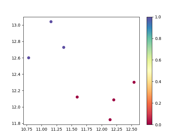
from sentence_transformers import SentenceTransformer
from umap import UMAP
from hdbscan import HDBSCAN
import matplotlib.pyplot as plt
import numpy as np

# load embedding model
embedding_model = SentenceTransformer("sentence-transformers/all-MiniLM-L12-v2")

# generate embeddings
texts = ['cats', 'dogs', 'elephants', 'birds', 'cars', 'trains', 'planes']
embeddings = embedding_model.encode(texts)

print(f'Number of embedded documents and their dimensions: {embeddings.shape}')

# reduce the embeddings dimensions
reduced_embeddings = UMAP(n_components=5, random_state=42).fit_transform(embeddings)

print(f'Number of embedded documents and their reduced dimensions: {reduced_embeddings.shape}')

# create an hdbscan object and fit the model to the data
cluster_labels = HDBSCAN(min_cluster_size=2, metric='euclidean').fit_predict(reduced_embeddings)

# get the number of clusters (excluding noise points labeled as -1)
n_clusters = len(set(cluster_labels)) - (1 if -1 in cluster_labels else 0)
n_noise = list(cluster_labels).count(-1)

print(f'Number of clusters: {n_clusters}')
print(f'Number of noise points: {n_noise}')

# print cluster results
for cluster_id in set(cluster_labels):
    if cluster_id == -1:
        print(f"\nNoise points:")
    else:
        print(f"\nCluster {cluster_id}:")
    
    cluster_indices = np.where(cluster_labels == cluster_id)[0]
    for index in cluster_indices:
        print(f'- {texts[index]}')

# plot the results (using first 2 components for visualization)
plt.figure(figsize=(10, 8))
scatter = plt.scatter(reduced_embeddings[:, 0], reduced_embeddings[:, 1], 
                     c=cluster_labels, cmap='Spectral', s=100)
plt.colorbar(scatter)
plt.title('HDBSCAN Clustering Results')
plt.xlabel('UMAP Component 1')
plt.ylabel('UMAP Component 2')

# annotate points with text labels
for i, text in enumerate(texts):
    plt.annotate(text, (reduced_embeddings[i, 0], reduced_embeddings[i, 1]),
                xytext=(5, 5), textcoords='offset points', fontsize=9)

plt.tight_layout()
plt.savefig('hdbscan_cluster_plot.png', dpi=300, bbox_inches='tight')
print("\nPlot saved as 'hdbscan_cluster_plot.png'")

Run the Python script:

$ python3 clustering.py

Output:

Number of embedded documents and their dimensions: (7, 384)

Number of embedded documents and their reduced dimensions: (7, 5)

Number of clusters: 2
Number of noise points: 0

Cluster 0:
- cats
- dogs
- elephants
- birds

Cluster 1:
- cars
- trains
- planes

Plot saved as 'hdbscan_cluster_plot.png'

Chart of the clusters: hdbscan_cluster_plot.png
Clusters Plot